Getting Started

This guide will go over the basic concepts of ndonnx and how to get started with the library.

Array Programming

ndonnx will feel familiar to users of libraries like NumPy since it implements a superset of the Array API standard. The complete Array API specification can be found elsewhere. Additional parts of the API specific to ndonnx are listed here.

Creating Arrays

ndonnx arrays can be instantiated from NumPy arrays, scalars or Python lists. Unlike most other libraries, ndonnx arrays can also be created only from a shape and data type. While these arrays don’t contain any data, they are used to trace computation graphs to facilitate ONNX export. This is discussed in more detail in the ONNX Export section below.

import ndonnx as ndx

# Initializing an array with data
a = ndx.asarray([1, 2, 3])

# Initializing an array with shape and data type
b = ndx.argument(shape=(3,), dtype=ndx.float64)

# Shapes can be symbolic using string dimensions
c = ndx.argument(shape=("N", "M"), dtype=ndx.utf8)

The ndonnx namespace

The top-level ndonnx namespace contains various functions such as ndonnx.sum that are mandated by the Array-API standard. Additional functions that go beyond the standard may be found in the ndonnx.extensions module.

import ndonnx as ndx
import ndonnx.extensions as nde

a = ndx.asarray([1, 2, 3])

# Functions and operators as defined by the Array API
b = ndx.min(a)
print(b) # array(data: 1, dtype=int64)
# Functions unique to ndonnx
c = nde.isin(a, [1, 3])
print(c) # array(data: [True, False, True], dtype=bool)

Slicing, Indexing, and Broadcasting

Slicing, indexing and broadcasting is also defined by the Array-API standard and will thus feel familiar to NumPy users.

import ndonnx as ndx

a = ndx.asarray([1, 2, 3])

# Indexing
b = a[0]
print(b) # Array(1, dtype=Int64)

# Slicing and broadcasting
c = a[1:3] + 4
print(c) # Array([6 7], dtype=Int64)

Data Types

ndonnx provides not only Array API compliant data types but also strings and nullable variants. You can find a full list here.

import ndonnx as ndx
import numpy as np

a = ndx.asarray(["foo", "bar", "baz"])
print(a.dtype) # Utf8

# Array of nullable integers
b = ndx.asarray(np.ma.masked_array([1, 2, 3], mask=[0, 1, 0]))
print(b) # Array([1 -- 3], dtype=NInt64)

# Mix and match nullable data types
c = b + ndx.asarray([1, 2, 3])
print(c) # Array([2 -- 6], dtype=NInt64)

Writing Array API compliant code

Writing code in a strictly Array API compliant fashion makes it instantly reusable across many different array backend libraries like NumPy, JAX, PyTorch and now ndonnx.

import ndonnx as ndx
import numpy as np

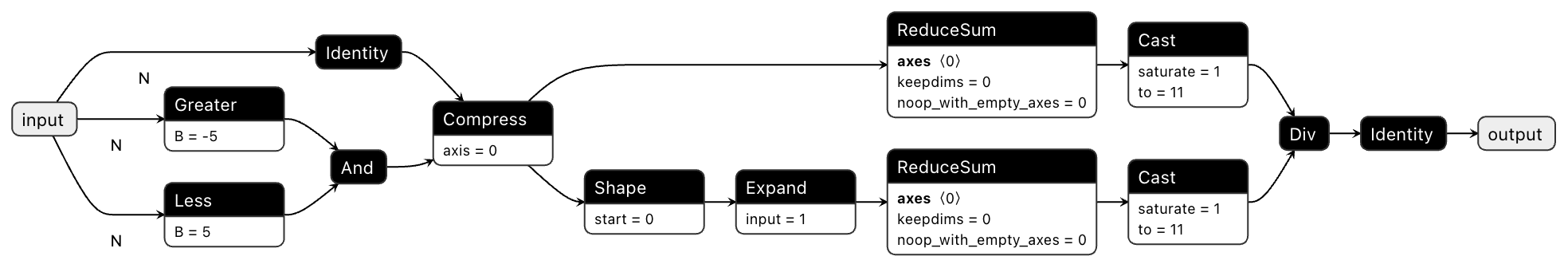
def mean_drop_outliers(a, low=-5, high=5):
    xp = a.__array_namespace__()
    return xp.mean(a[(low < a) & (a < high)])

np_result = mean_drop_outliers(np.asarray([-10, 0.5, 1, 4]))
onnx_result = mean_drop_outliers(ndx.asarray([-10, 0.5, 1, 4]))
np.testing.assert_equal(np_result, onnx_result.unwrap_numpy())

ONNX Export

ndonnx arrays do not need to hold data. They can instead be instantiated with only a shape and data type. This gives you the ability to persist the traced computation graph as an ONNX model and provide compatible input values only at inference time.

import ndonnx as ndx
import onnx

# Instantiate placeholder ndonnx array
x = ndx.argument(shape=("N",), dtype=ndx.float64)
y = mean_drop_outliers(x)

# Build and save my ONNX model to disk
model = ndx.build({"x": x}, {"y": y})
onnx.save(model, "mean_drop_outliers.onnx")

We can visualize this model using Netron.

Note

ndonnx will write versioned metadata in your ONNX model that may be used by downstream inference oriented libraries. You can find out more in the Inference Utilities section.